Distinction between Pearson and Spearman Correlations

Pearson correlation measures a linear relationship between X and Y, while Spearman correlation estimates a non-linear relationship. In some cases, the relationship between X and Y (e.g.  Bitrate and Quality) is strictly non-linear:

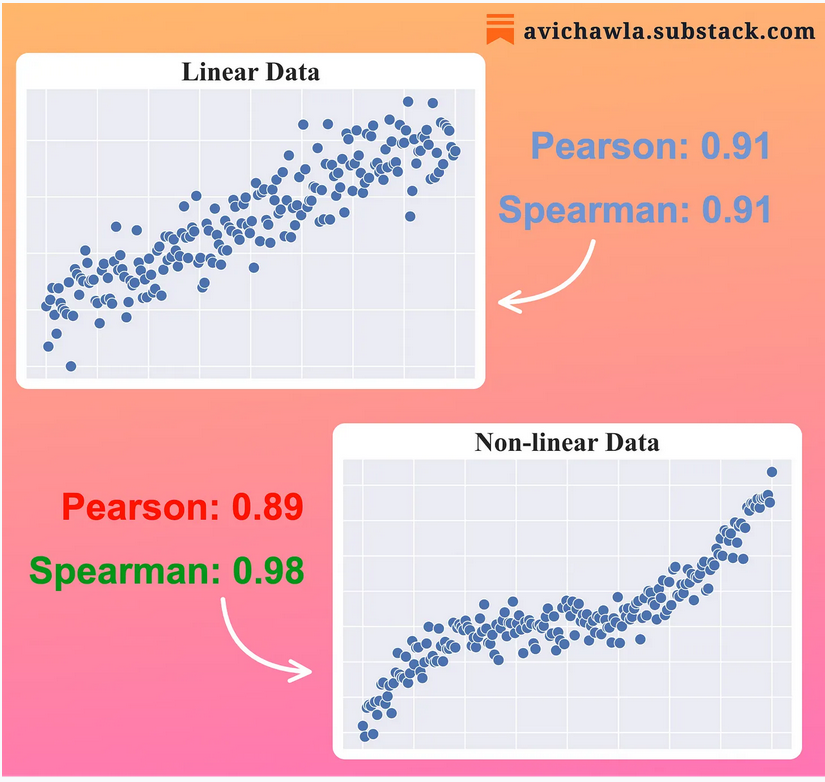
taken from https://avichawla.substack.com/p/the-limitation-of-pearson-correlation

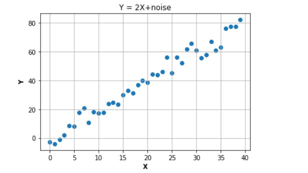
The following Python script shows how to compute Pearson and Spearman correlation coefficients:

import numpy as np
import scipy.stats
import matplotlib.pyplot as plt

# generate distorted linear data of Y = 2X
X=np.array(range(0,40))
Y = [ 2*x for x in X]
D = 4*np.random.randn(1,40)
Yd = np.array(Y + D)  # add nois
Yd=Yd[0]

fig, ax = plt.subplots()
plt.grid()
plt.title(‘Y = 2X+noise’)
ax.set_ylabel(‘Y’,fontdict=dict(weight=’bold’))
ax.set_xlabel(‘X’,fontdict=dict(weight=’bold’))
ax.scatter(X, Yd)

# Pearson correlation coefficient

scipy.stats.pearsonr(X, Yd)[0]

0.9858533253709376

# Spearman correlation coefficient

scipy.stats.spearmanr(X, Yd)[0]

0.9838649155722327

# generate distorted linear data of Y = X^2
Y1 = [ x*x for x in X]
D1 = 32*np.random.randn(1,40)
Yd1 = np.array(Y1 + D1)
Yd1=Yd1[0]

fig, ax = plt.subplots()
plt.grid()
plt.title('Y = X^2+noise')
ax.set_ylabel('Y',fontdict=dict(weight='bold'))
ax.set_xlabel('X',fontdict=dict(weight='bold'))
ax.scatter(X, Yd1)



scipy.stats.pearsonr(X, Yd1)[0]

0.9627985894542643

scipy.stats.spearmanr(X, Yd1)[0]

0.9904315196998127

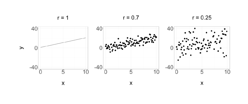
Appendix A: Examples of Pearson Correlation ‘r’

Appendix B: Linear Regression Equation

For input train {x_i} data and output {y_i} the coefficients of linear equation:  y = c₀ + c₁ * x  are determined as follows:

Python script to compute c₀ and c₁:

1.9718933743372042
3.091355148859236

Slava

23+ years’ programming and theoretical experience in the computer science fields such as video compression, media streaming and artificial intelligence (co-author of several papers and patents).

the author is looking for new job, my resume

Donate

Related posts:

Implementation of Anti-aliasing Filter in Downscaling VLC Media Player from Command Prompt (Alternative of ffmpeg) Hawking Radiation Atheism and materialism in the age of the the Enlightenment Useful Commands of Python ‘pip Stability of System Linear Equations and Condition Number